Beyond Pure Vectors: Implementing High-Precision Hybrid Search Natively inside Postgres

We observed a 500ms synchronization lag when separating our storage engine from an external search cluster, which causes broken user experiences when resolving exact alphanumeric queries. Dense embeddings capture abstract semantic meaning but fail at exact keyword matching, causing queries for precise serial numbers like X-992-B, legacy product SKUs, or industry-specific jargon like Kubernetes to return incorrect results.

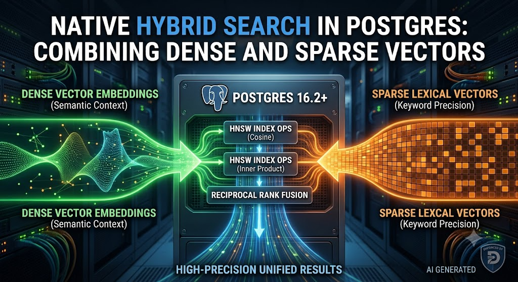
We reject the industry reaction of deploying separate enterprise search clusters (such as Elasticsearch or OpenSearch) or specialized vector databases alongside the primary database. This architecture forces the maintenance of two separate data stores, creates eventual consistency issues, doubles infrastructure costs, and introduces complex synchronization pipelines. We enforce high-precision hybrid search natively inside PostgreSQL, combining dense semantic vector embeddings with neural sparse lexical vectors (sparsevec) within a single ACID-compliant transactional boundary.

graph TD
    UserQuery[User Search Query] --> Embedder[Application Embedding Pipeline]
    Embedder -->|"Dense Model (e.g., OpenAI)"| DenseV[Dense Vector vector 1536]
    Embedder -->|"Sparse Model 
(e.g., SPLADE)"| SparseV[Sparse Vector sparsevec 32000]
    DenseV --> Router[Postgres Engine]
    SparseV --> Router
    Router -->|"1: Contextual Match"| HNSW_Dense[HNSW Index vector
_cosine_ops]
    Router -->|"2: Exact Lexical Match"
| HNSW_Sparse[HNSW Index sparsevec_inner
_product_ops]
    HNSW_Dense --> DenseScore[Dense Rank]
    HNSW_Sparse --> SparseScore[Sparse Rank]
    DenseScore --> RRF[Reciprocal Rank 
Fusion Function]
    SparseScore --> RRF
    RRF --> FinalResult[High-Precision 
Unified Results]

Step 1: Designing the Dual-Vector Schema

We build a table structure that stores raw entity data alongside two distinct vector formats: a standard 1536-dimension dense vector for abstract semantic context, and a 32,000-dimension sparsevec column representing neural lexical term mappings generated via models like SPLADE or BGE-M3.

-- Enable the pgvector extension (Requires v0.7.0+ for sparsevec support)
CREATE EXTENSION IF NOT EXISTS vector;

-- Create high-precision product catalog table
CREATE TABLE products (
    id SERIAL PRIMARY KEY,
    sku VARCHAR(50) UNIQUE NOT NULL,
    title TEXT NOT NULL,
    description TEXT,
    category VARCHAR(100),
    
    -- 1536-dimension dense embedding for semantic context
    dense_embedding vector(1536),
    
    -- 32,000-dimension sparse vector for lexical precision
    sparse_embedding sparsevec(32000)
);

Engineering Note: The sparsevec(32000) type defines the total maximum vocabulary size of the sparse embedding model. PostgreSQL dynamically optimizes disk storage, writing data exclusively for elements containing non-zero weights to maximize memory and disk efficiency.

Step 2: Dual-HNSW Index Strategy for Performance

To maintain rapid retrieval times as the dataset scales into millions of rows, we deploy two distinct Hierarchical Navigable Small World (HNSW) graphs.

-- Create an HNSW index using Cosine Distance for dense vector search
CREATE INDEX idx_products_dense_hnsw ON products USING hnsw (dense_embedding vector_cosine_ops)
WITH (m = 16, ef_construction = 64);

-- Create an HNSW index using Inner Product for sparse lexical search
CREATE INDEX idx_products_sparse_hnsw ON products USING hnsw (sparse_embedding sparsevec_ip_ops)
WITH (m = 16, ef_construction = 64);

We score sparse vector matches using Inner Product (sparsevec_ip_ops), as the magnitude represents the absolute keyword and term weight generated by lexical models.

Step 3: Implementing Reciprocal Rank Fusion (RRF) Natively

We observed that direct scalar addition ($DenseScore + SparseScore$) fails because the scale of cosine distance differs fundamentally from sparse inner-product scaling. We enforce Reciprocal Rank Fusion (RRF) to evaluate the relative position (rank) of an item in both result sets instead of its raw score.

The formula for the RRF score of a document $d$ is:

Where $M$ is the set of search strategies (Dense and Sparse), $r_m(d)$ is the rank of document $d$ within strategy $m$, and $k$ is a constant smoothing factor set to 60 to prevent low-ranked items from heavily skewing the results.

We execute this hybrid search in a single database round-trip using a custom SQL function:

CREATE OR REPLACE FUNCTION hybrid_neural_search(
    query_dense vector,
    query_sparse sparsevec,
    match_limit INT DEFAULT 10,
    smoothing_k INT DEFAULT 60
)
RETURNS TABLE (
    id INT,
    sku VARCHAR,
    title TEXT,
    category VARCHAR,
    combined_score NUMERIC
) AS $$
WITH dense_results AS (
    SELECT 
        id, 
        ROW_NUMBER() OVER (ORDER BY dense_embedding <=> query_dense) as rank
    FROM products
    ORDER BY dense_embedding <=> query_dense
    LIMIT (match_limit * 3)
),
sparse_results AS (
    SELECT 
        id, 
        -- <#> operator returns negative inner product to sort highest score first
        ROW_NUMBER() OVER (ORDER BY sparse_embedding <#> query_sparse) as rank
    FROM products
    ORDER BY sparse_embedding <#> query_sparse
    LIMIT (match_limit * 3)
)
SELECT 
    p.id, 
    p.sku, 
    p.title, 
    p.category,
    COALESCE(1.0 / (smoothing_k + d.rank), 0.0) + 
    COALESCE(1.0 / (smoothing_k + s.rank), 0.0) AS combined_score
FROM products p
LEFT JOIN dense_results d ON p.id = d.id
LEFT JOIN sparse_results s ON p.id = s.id
WHERE d.id IS NOT NULL OR s.id IS NOT NULL
ORDER BY combined_score DESC
LIMIT match_limit;
$$ LANGUAGE sql STABLE;

Step 4: Optimization Guidelines

When running native hybrid search in high-throughput environments, we adjust database configurations beyond default out-of-the-box settings.

Production Verification Checklist

• Verify Simultaneous Index Execution: Run EXPLAIN ANALYZE on hybrid queries to ensure both idx_products_dense_hnsw and idx_products_sparse_hnsw execute simultaneous index scans without falling back to sequential table space searches.
• Warm Your Graphs: Preload both dense and sparse HNSW graphs into the PostgreSQL buffer cache by executing dummy vector scans during the application boot sequence.
• Partitioning Strategy: If the dataset spans tens of millions of rows, partition tables by a logical boundary like category or tenant_id.
• Local Indexing: Deploy local HNSW indexes across these partitions to keep individual graph indexes compact and fast.

We have not fully resolved two operational behaviors:

• We are currently hacking around a vocabulary boundary constraint, forcing a pre-filtering step inside the application layer when SPLADE generates token IDs exceeding our 32000-dimension schema limit, rather than using a dynamic mapping logic within Postgres.
• We observed severe query throughput inversion on collections smaller than 1 million rows when attempting to use the diskann index type, meaning we enforce HNSW purely for sub-scaling workloads due to the introduced quantization decoding floor.

We are now validating the diskann index type made available via the pgvectorscale extension. This extension allows us to execute disk-backed graph traversal, transitioning our vector operations from being constrained by physical RAM allocation metrics to being gated by NVMe storage IOPS. By enforcing Statistical Binary Quantization (SBQ) on high-dimensional vectors, DiskANN maintains significant recall accuracy while shrinking the working set footprint to approximately 8.2% of its uncompressed layout. This engineering path complements our existing native hybrid search strategy, providing a scale-out mechanism when individual vector collections exceed physical hardware bounds. We base our implementation on the foundational DiskANN research.